Analysing Crossoak
Category: misc
A friend had a theory that photography, and therefore by extension c r o s s o a k is a window into my mental well being. So I did some digging which I'm capturing here (and which is in all probability a much bigger insight into my head...). If you have a similar theory, you might think the conclusion tells you quite a lot. If you don't it won't.
Getting the data
First off, let's grab some data from Wordpress, the blog platform that currently powers c r o s s o a k.
from wordpress_xmlrpc import Client, WordPressPost
from wordpress_xmlrpc.methods.posts import GetPosts
from bs4 import BeautifulSoup
import json

wp = Client(BLOG_URL + '/xmlrpc.php')
This gets a reference to wp which we can use to query wordpress, for example this code:
post_data = {}
# get pages in batches of 20
offset = 0
increment = 20
while True:
    posts = wp.call(
        GetPosts({'number': increment, 'offset': offset})
    )
    if len(posts) == 0:
        break  # no more posts returned
    for post in posts:
        post_data[post.id] = {"title": post.title,
           "date": post.date.strftime("%Y%m%d"),
           "img_count": count_images(post)}
    offset = offset + increment
will get some basic data on all the posts in the blog. In the above count_images uses BeautifulSoup to parse post content to count img tags like this:
def count_images(post):
    soup = BeautifulSoup(post.content, 'lxml')
    imgs = soup.findAll('img')
    return len(imgs)
So you don't have to keep querying the site, you can save to a local file. For example, to export as JSON with:
with open('wp_data.json', 'w') as outfile:
    json.dump(post_data, outfile)
which looks something like this:
{
    "4444": {
        "title": "Wandering Around Wasdale",
        "date": "20181027",
        "img_count": 5
    }
}
where 4444 is the post id which you can use to reference the post on the blog with https://www.aiddy.com/crossoak?p=4444.
Exploring the data
To analyse the content we'll use Pandas and Seaborn.
import json
import pandas as pd
import numpy as np
import seaborn as sns
import matplotlib.pyplot as plt

# load JSON file with our Wordpress data
with open('wp_data.json') as json_data:
    d = json.load(json_data)

# convert to a DataFrame
df = pd.DataFrame(d)
df = df.transpose()
df.reset_index(inplace=True)
df.rename(columns={'index': 'id'}, inplace=True)
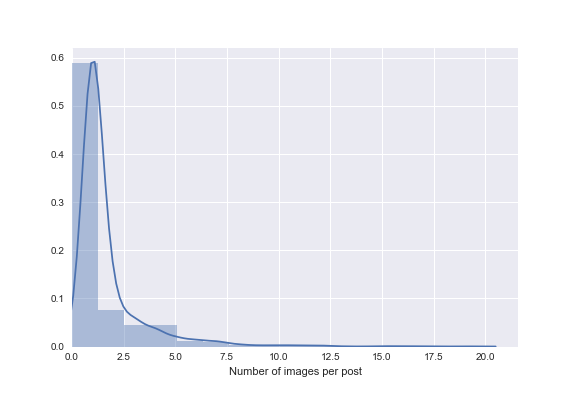
Which we can then use to visualize the distribution of the number of images per post.
sns.distplot(df.img_count, kde_kws={"bw":.5}, bins=15)
sns.plt.xlim(0, None)
sns.plt.xlabel('Number of images per post')
To delve a bit data, we'll augment the data, breaking out the date with year, month, day and weekday and counting words and characters in the titles...
df['date'] = pd.to_datetime(df['date'], format='%Y%m%d')
df['year'] = df['date'].dt.year
df['month'] = df['date'].dt.month
df['day'] = df['date'].dt.day
df['weekday'] = df['date'].dt.weekday
df['title_words'] = df['title'].map(lambda x: len(str(x).split()))
df['title_chars'] = df['title'].map(lambda x: len(x))
df['title_wordlength'] = df['title_chars'] - df['title_words']
...and calculate summaries using groupby for counts of posts and the total number of images:
# get summarized views
df_imgs = df.groupby([df.year, df.month]).img_count.sum()
df_posts = df.groupby([df.year, df.month]).id.count()
df_imgs = pd.DataFrame(df_imgs)
df_imgs.reset_index(inplace=True)
df_posts = pd.DataFrame(df_posts)
df_posts.reset_index(inplace=True)

df_summary = pd.merge(df_imgs, df_posts, on=['month', 'year'])
Comparing the DataFrames for the original data imported from JSON in df:
| id | date | img_count | title | year | month | day | weekday | title_chars | title_words | title_wordlength | |
|---|---|---|---|---|---|---|---|---|---|---|---|
| 0 | 100 | 2009-10-28 | 1 | Last game | 2009 | 10 | 28 | 2 | 9 | 2 | 7 |
| 1 | 1000 | 2005-10-23 | 1 | Alice\'s Jugs | 2005 | 10 | 23 | 6 | 12 | 2 | 10 |
| 2 | 1001 | 2005-10-23 | 1 | Padstow Sunrise | 2005 | 10 | 23 | 6 | 15 | 2 | 13 |
| 3 | 1002 | 2005-10-23 | 1 | Rock at Night | 2005 | 10 | 23 | 6 | 13 | 3 | 10 |
| 4 | 1003 | 2005-10-23 | 1 | Padstow Sunset | 2005 | 10 | 23 | 6 | 14 | 2 | 12 |
and the view in df_summary:
| year | month | img_count | id | |
|---|---|---|---|---|
| 0 | 2005 | 5 | 50 | 50 |
| 1 | 2005 | 6 | 17 | 17 |
| 2 | 2005 | 7 | 8 | 8 |
| 3 | 2005 | 8 | 21 | 21 |
| 4 | 2005 | 9 | 7 | 7 |
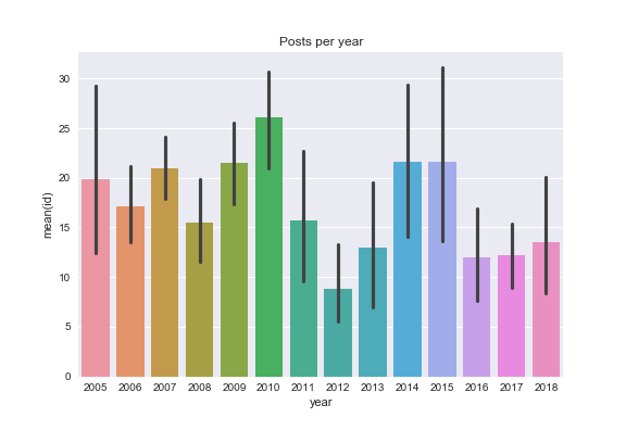
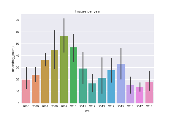
Now we can dig into: posts & images per year...
sns.barplot(df_summary['year'],df_summary['id'])
sns.barplot(df_summary['year'],df_summary['img_count'])
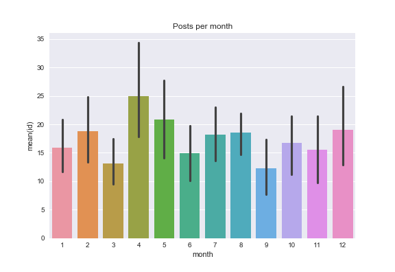
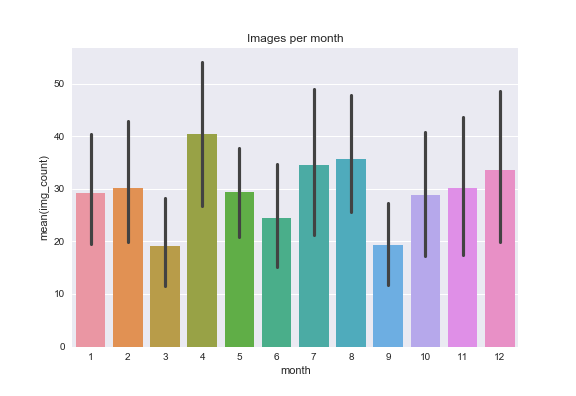
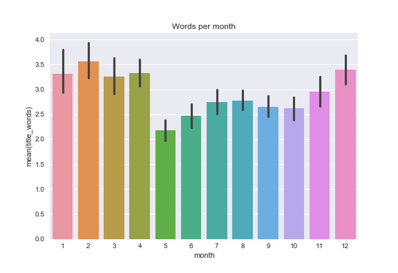
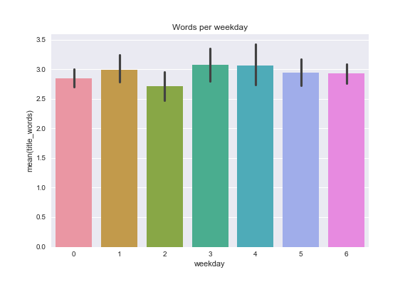
And per month:
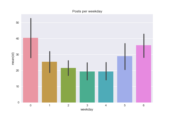
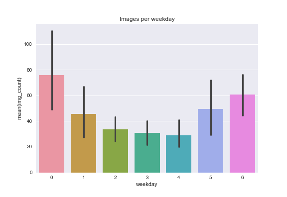
And per weekday:
Using the summary data we can also explore correlations between fields with a pair plot:
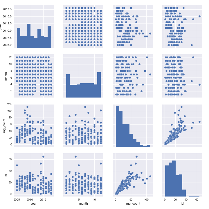
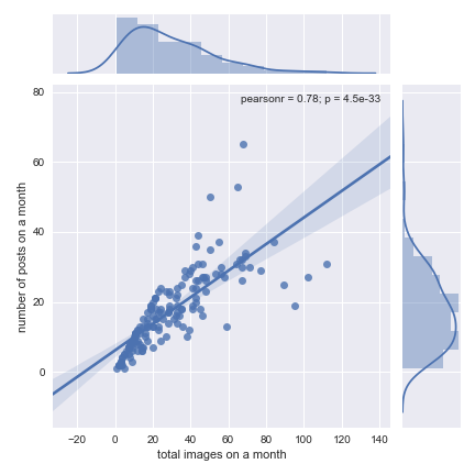
or look at the correlation between number of posts and number of images per month
jp = sns.jointplot(df_summary['img_count'], df_summary['id'], kind='reg')
jp.set_axis_labels('total images on a month', 'number of posts on a month')
We can also play around with the words used in titles:
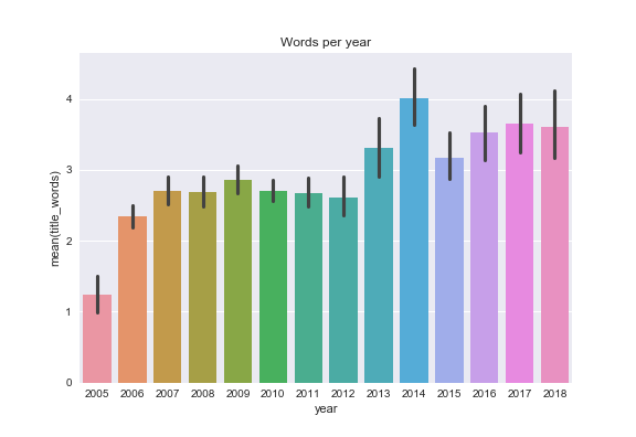
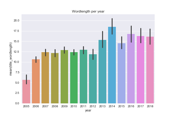
and also see if I used longer or shorter words in post titles over the years c r o s s o a k has been published
Conclusions
So what have we learnt from the excursion into the data lurking behind c r o s s o a k?
- 2012 was a low year for both posts and images posted. The number of posts recovered slightly in 2016-2018 but not the number of images (more posts have only one image on average).
- April is when I post most
- I post on weekend's and Fridays more than midweek
- I use the fewest words in post titles in May
- Over the years I've used more words and longer words in post titles
- This is the kind of thing you do on a dark autumn evening in the northern hemisphere. Apparently it's why Scandinavia has so many tech start-ups (relative to population).